common evaluation ways for binary classification model
Confusion Matrix and Table of Confusion
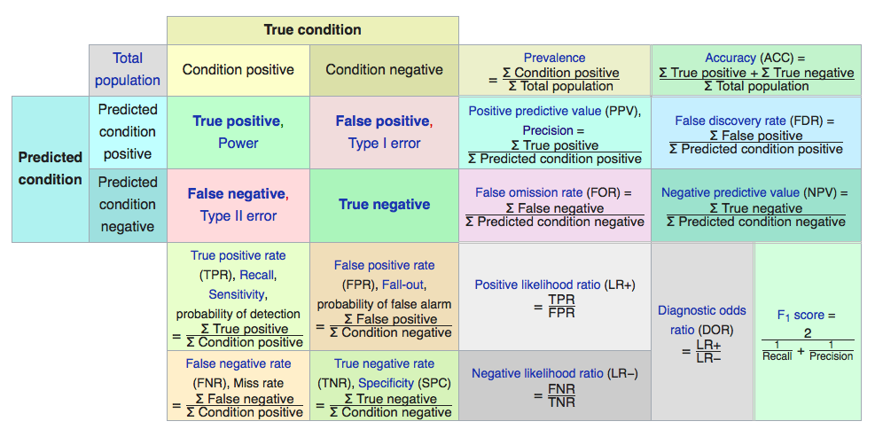
Confusion matrix is a specific table layout that allows visualization of the performance of an algorithm, typically a supervised learning one. Here is a basic example:
Here is a prediction result from a classification model.
| prediction | 1 | 2 | 3 | 1 | 1 | 1 | 3 |
|---|---|---|---|---|---|---|---|
| true | 1 | 2 | 2 | 2 | 3 | 2 | 1 |
Use confusion matrix to interpret it and we get:
| 1 | 2 | 3 | True | |
|---|---|---|---|---|
| 1 | 1 | 2 | 1 | |
| 2 | 0 | 1 | 0 | |
| 3 | 1 | 0 | 0 | |
| Prediction |
To interpret this matrix, take look at the forth row. This mean there’s one time that we predict 1 into 3. Then we introduction a defination called table of confusion. It’s a table with two rows and two columns that reports the number of false positives, false neagatives, true positives and true negatives. Take look at our next example.
| actual 1 | actual other than 1 | |
|---|---|---|
| predict 1 | 1(true positive) | 3(false positive) |
| predict other than 1 | 1(true negative) | 2(false negative) |
So far everything is still simple. We introduce four new concepts to evaluate the performance of our model.

Although all these concepts and formula are still not so hard to understand, when and which concept we should use becomes complicated. I will discuss the main differences, advantages and disadvantages of each measurement, and how to combine them together to evaluate model performance.
F1 Score
(Positive Predictive Value) Precision represents “how many selected items are relevant”, and (True Positive Rate) Recall represents “how many relevant items are selected”. The former observes TP number in chosen dataset and the latter observes TP in original dataset. We usually use the harmonic average of both to measure test’s accuracy (F1 score).
$$F1 = frac{2 times recall times precision}{recall + precision}$$
The reason we use harmonic average is that the closer precision and recall are, the more reliable our measurement is. We can relate this formula to dice similarity coefficient, which is used for comparing the similarity of two samples.
The main drawback of using F-score is listed below:
- It focus on only one class. It reveals the discriminative power of each feature independently from others, but it does not indicate anything on the combination of both features.
- It’s biased to the majority class. For example if there are 90% male candidates and 10% female candidates and our model can simply predict all candidates are male, which will give us 100% recall and 90% precision.
- It doesn’t take into account the True Negative. TN can change arbitrarily without changing F-measure.
ROC, AUC and Informedness
A ROC space depicts relative trade-offs between true positive and false positive. In binary classification , we predict a score for each instance. Given a threshold parameter T, the instance is classified as positive if X > T and negative otherwise. Usually as threshold gets looser, TPR increases and FPR increases as well. Therefore, a ROC space is defined by FPR and TPR as x and y axes at various threshold settigs. We usually use AUC(Area Under the Curve) to summarize the ROC curve.
AUC can be interpret as the probability that the classifier will assign a higher score to a randomly chosen positive example than to a negative example. The main drawback of using AUC is listed below:
- It doesn’t work well with small dataset, since it generlizes a step function into a continuous curve.
- It ignores the fact that the curve is about the tradeoffs between the different systems.
- AUC doesn’t tell you the costs of different kinds of errors. It will treat a 10000 dollar fraud the same as a 10 dollar fraud.
- It does not account for false negative cases.
- It’s also biased to the total amount of positive and negative cases.
Accuracy
Accuracy is one of the most common used stastics data. The formula is pretty clear so let’s go straight to its drawback. The main disadvantage is that iff TN is large, the influence of TP becomes minor.
Matthew Correlation Coefficient
frac{sum_{n} (P_n - overline{R}) (S_n - overline{S})}{sqrt{sum_n (P_n - overline{P})^2 sum_n (P_n - overline{P})^2}}
$$
where $overline{P}$ represents the mean of prediction, $P_n$ represents the nth prediction, $overline{S}$ represents the mean of observation and $S_n$ represents the nth obeservation.
The fomula above can be transformed to following one, which is what we commonly see.
Matthew Correlation Coefficient use the correlation between the prediction and observation to evaluate the model performance. It’s so far seen as one of the best measurements for binary classification, since it takes into account the balance ratios of the four confusion matrix categories.
Conclusion
Generalize the confusion matrix trades off some features in data. Under different circumstances, we evaluate four confusion matrix categories differently. Each measurement pays attention to some particular aspects in dataset. Therefore, it’s important to know when and how to use these tools to get a comprehensive understanding about our model.


